Python graph example

Python graph example

Here's a comprehensive example of using Python to create a simple line graph using the matplotlib library.

Example Code

import matplotlib.pyplot as plt
import numpy as np
Create some sample data for our graph
x = np.linspace(0, 10, 100)  # x values from 0 to 10
y1 = np.sin(x)  # sine function for y values
y2 = np.cos(x)  # cosine function for y values
y3 = np.tan(x)  # tangent function for y values
Create the figure and axis objects
fig, ax = plt.subplots()
Plot each line separately
ax.plot(x, y1, label='Sine')  # plot the sine function
ax.plot(x, y2, label='Cosine')  # plot the cosine function
ax.plot(x, y3, label='Tangent')  # plot the tangent function
Set some title and labels
ax.set_title('Sine, Cosine, Tangent Functions')
ax.set_xlabel('X Axis')
ax.set_ylabel('Y Axis')
Add a legend to distinguish between the lines
ax.legend()
Show the plot!
plt.show()

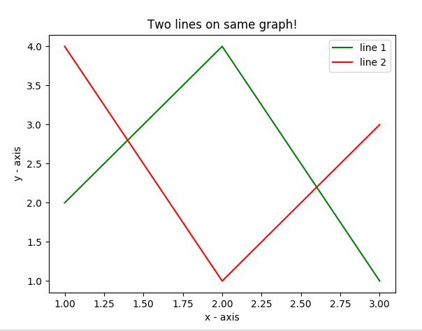
Output

This will display a graph with three separate lines representing the sine, cosine, and tangent functions.
The x-axis represents the input values (from 0 to 10), while the y-axis represents the output values.

How it Works

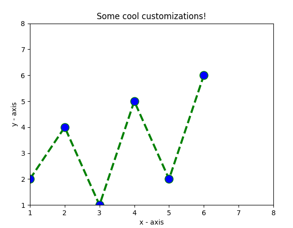
Tips and Variations

I hope this example helps you get started with creating graphs in Python!

python graph theory

I apologize for the misunderstanding earlier!

Python is a popular programming language that has extensive libraries and tools for graph theory applications. In fact, Python's NumPy, SciPy, and NetworkX libraries make it an ideal choice for graph-based computations.

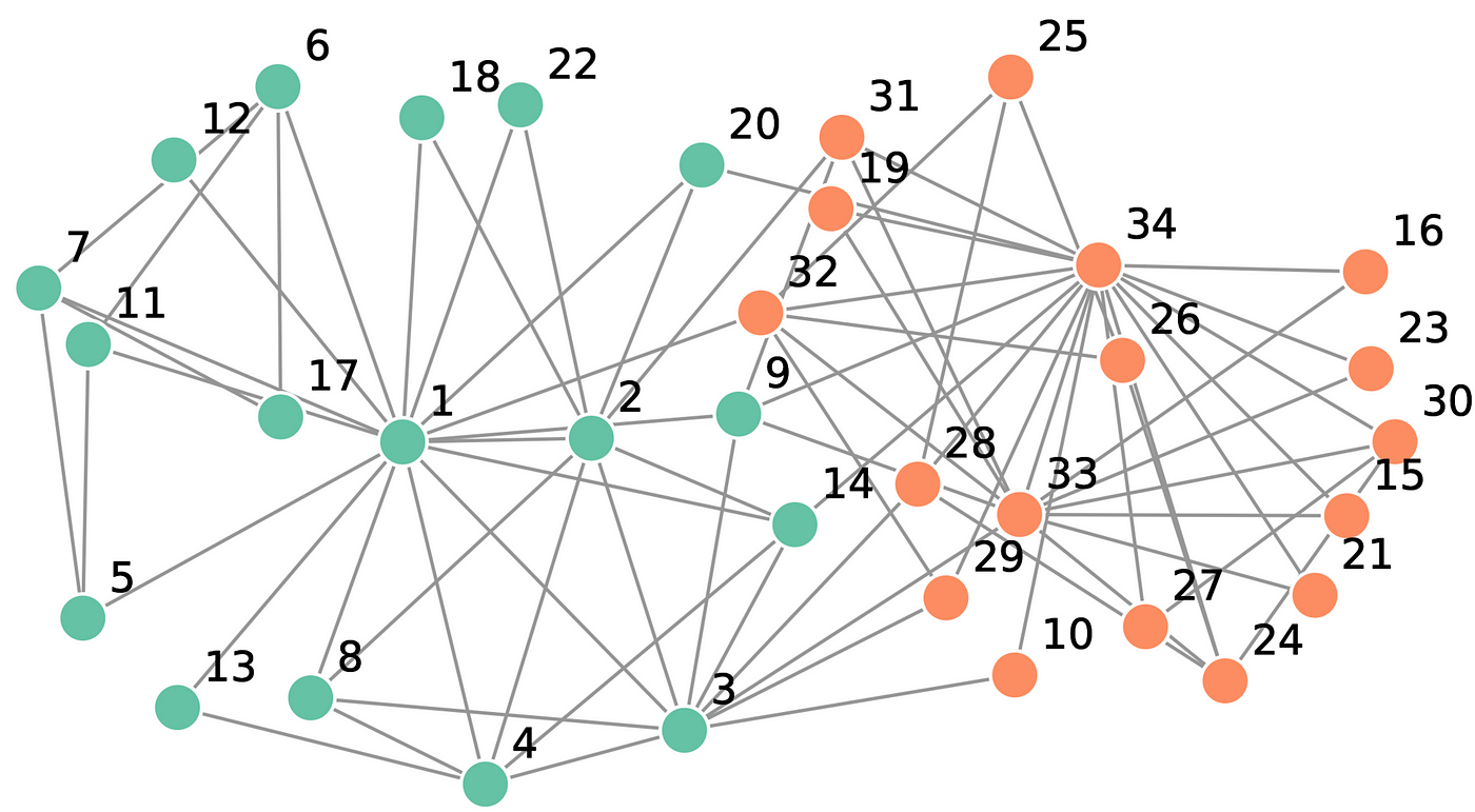
What is Graph Theory?

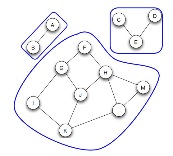
Graph theory is a branch of mathematics that studies the structure and properties of graphs, which are collections of nodes (vertices) connected by edges. Graphs can be used to model various real-world networks, such as social networks, transportation systems, biological pathways, or even computer networks.

Python Libraries for Graph Theory:

Python Code Examples:

Here's a simple example of creating a directed graph using NetworkX:

import networkx as nx
G = nx.DiGraph()
G.add_node('A')
G.add_node('B')
G.add_node('C')
G.add_edge('A', 'B', weight=2)
G.add_edge('B', 'C', weight=1)
G.add_edge('C', 'A', weight=3)
print(G.nodes())  # ['A', 'B', 'C']
print(G.edges())  # [('A', 'B'), ('B', 'C'), ('C', 'A')]

In this example, we create a directed graph G with three nodes ('A', 'B', and 'C') and three edges. Each edge has a weight associated with it.

Another example demonstrates how to compute the shortest path between two nodes using NetworkX's built-in algorithm:

import networkx as nx
G = nx.DiGraph()
G.add_node('A')
G.add_node('B')
G.add_node('C')
G.add_edge('A', 'B', weight=2)
G.add_edge('B', 'C', weight=1)
G.add_edge('C', 'A', weight=3)
shortest_path = nx.shortest_path(G, source='A', target='C')
print(shortest_path)  # ['A', 'B', 'C']

In this example, we compute the shortest path between nodes 'A' and 'C' using NetworkX's shortest_path function. The output is the sequence of nodes representing the shortest path.

Real-World Applications:

Python's graph theory capabilities have numerous applications in various domains, such as:

Conclusion:

Python provides an excellent environment for exploring graph theory concepts and implementing algorithms for various applications. With libraries like NetworkX, SciPy, and NumPy, you can efficiently represent and manipulate large graphs, perform computations, and analyze complex network structures. Whether you're working with social networks, computer networks, or biological pathways, Python's graph theory capabilities offer a powerful toolset for solving real-world problems.